Case Tree Analyses Case tree plot analyses
Case tree plots are useful for visualizing and analyzing small clusters of zoonotic disease with limited human to human potential. Examples include MERS-CoV and Ebola.
Basic reproduction number
What is the basic reproduction number?
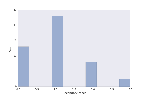
The basic reproduction number, also called R0, is the average number of secondary cases each case produces in a fully susceptible population. In order for an outbreak to sustain itself, R0 must be greater than 1. The higher the R0, the more infectious the disease.
For most outbreaks, R0 must be estimated. Case tree plots have the advantage of showing the exact number of secondary cases per source case.
Example
For this example, we’ll use data from the MERS-CoV packaged with epipy. You may need to change the path below. To start, first build out the graph. Then simply call reproduction_number(), which will return a series object, and a histogram of the R0s. The function has an option to exclude index cases (index_cases=False), which is useful if you want to calculate the human to human reproduction number without considering zoonotically acquired cases.
import epipy
import pandas as pd

data = epipy.generate_example_data(cluster_size=10, outbreak_len=100, clusters=10, gen_time=5)
If you’re working with case tree plots, you can get the graph from the case_tree_plot function.
G, fig, ax = epipy.case_tree_plot(data, cluster_id='Cluster', case_id='ID', date_col='Date', color='Cluster', gen_mean=5, gen_sd=2)
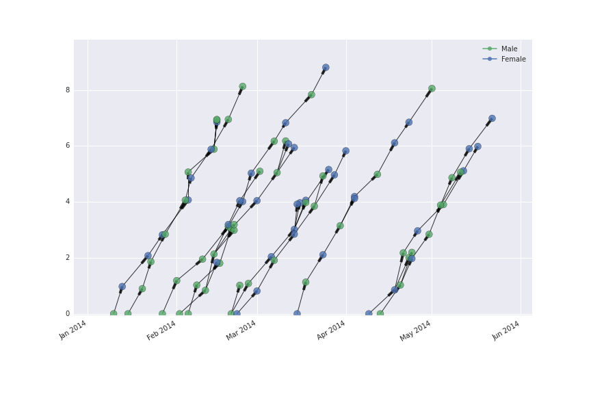
But if you want don’t want to produce the plot, you can get the same thing using the build_graph function.
G = epipy.build_graph(data, 'Cluster', 'ID', 'Date', 'Cluster', 5, 2)
You can then use the graph to assess the reproduction number. You may choose whether or not to include the index cases in the calculation.
R, fig, ax = epipy.reproduction_number(G, index_cases=True, plot=True)
The series object, R in the above example, can be manipulated further.
print R.describe()
The R variable returns:
count    101.000000
mean       1.000000
std        1.296148
min        0.000000
25%        0.000000
50%        0.000000
75%        2.000000
max        5.000000
dtype: float64
And the figure returns:
Generation analyses
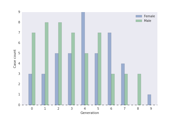
Epidemiologists may also be interested in how the disease changes from one generation to the next. Are cases acquired from animals more severe than human acquired cases? Does severity decrease as the disease passes from person to person? Are index cases more likely to be men? The generation_analysis() function returns a table of case attributes by generation, as well as an optional bar graph.
Example
fig, ax, table = fig, ax, table = epipy.generation_analysis(G, attribute='sex')
The table variable returns:
sex by generation
sex         Female  Male  All
generation
0                3     7   10
1                3     8   11
2                5     8   13
3                5     7   12
4                9     5   14
5                5     7   12
6                7     3   10
7                4     3    7
8                0     3    3
9                1     0    1
All             42    51   93
And the figure returns a histogram of number of cases at each generation, by attribute: